Getting started
Table of contents
MCMC Recap
In Bayesian inference, one commonly aims to compute a posterior using a prior and likelihood. However, the exact value of the posterior probability is often intractable. Nonetheless, it is possible to construct an approximation via sampling.
MCMC (Markov chain Monte Carlo) is a group of sampling algorithms, generating stochastic Markovian draws from an unknown (posterior) distribution.
Find a short, intuitive explanation in this blog post.
Or a more in-depth explanation of Bayesian Inference with Hamiltonian Monte Carlo in this video, reviewing this paper.
Algorithm
General steps
- Define a proposal distribution \(q(x, x_t)\) and a length scale parameter (epsilon).
- Pick an initial state \(x_0\)
- Iteratively: a. Draw a sample \(x^\star\) from the proposal distribution. b. Calculate an acceptance probability (a simple one would be \(p = \min (\frac{q(x^\star)}{q(x_t)}, 1)\)). c. update the state, if sample accepted \(x_{t+1}=x^\star\), otherwise \(x_{t+1}=x_t\)
A simple MCMC (i.e., the Metropolis-Hastings algorithm) explores the space by moving through spaces of relatively high probability. In high dimensional spaces (where spaces of very low probability are common), MH would perform poorly, or at least, very inefficiently.
Comes HMC..
Stan’s MCMC
The Hamiltonian Monte Carlo (HMC) algorithm offers a better solution for high dimensions. HMC introduces an auxiliary variable (\(y\)) which, via motion equations borrowed from Newtonian mechanics, allows exploring a multidimensional space more efficiently. The main problem is solving the Hamiltonian equations efficiently. HMC uses 3 parameters (read more here), which Stan automatically optimizes based on warmup sample iterations or dynamically adapts using the no-U-turn sampling (NUTS) algorithm. Nicely eliminating the need for user-specified tuning parameters.
Pay attention, Hamiltonian algorithms still have limitations.
- HMC requires continuous parameter spaces (i.e., no discrete parameters).
- Multimodal targets, among other weirdly shaped distributions, are often problematic to sample from.
More than sampling
In addition to performing full Bayesian inference via posterior sampling, Stan also can perform optimization & Variational inference. But we won’t get into it here…
Syntax
A Stan program defines a statistical model through a conditional probability function \(p(\theta \| y, x)\). It models: (1) \(\theta\), a sequence of unknown values (e.g., model parameters, latent variables, missing data, future predictions) and (2) \(y\), a sequence of known values - including \(x\), a sequence of predictors and constants (e.g., sizes, hyperparameters).
General
- Comments in Stan follow a double backslash
\\. - Every line ends with a semicolon
;. - Stan supports arithmetic and matrix operations on expressions as well as loops & conditions.
- Stan indexing starts at 1.
Program blocks
Stan programs feature several distinct parts named blocks:
functions{}contains user-defined functionsdata{}declares the required data for the model, i.e., the components of the observational spacetransformed data{}defines the changes to the format or structure of the data, as required by the model (if required)parameters{}declares the (unconstrained version of the) model’s parameters, which are sampled or optimized.transformed parameters{}defines the changes to the format or structure of the parameters, as required by the model (if required)model{}defines the log probability functiongenerated quantities{}derives user-defined quantities based on the data and sampled parameters
All of the blocks are optional, but when used - the blocks appear in the above order. Commonly, one uses at least the data, parameters, and model blocks in a basic Stan program (see the Bernoulli example).
Program flow (based on the block design)
- Every chain executes the
data{},transformed data{}, andparameters{}blocks. Reads data into memory, validate them, and initializes the parameters values. - The multistep sampling * process iteratively evaluating the negative log probability function and its gradient according to the current parameters values. Each step executes the
transformed parameters{}and themodel{}blocks. A Metropolis-accept/reject step determines the new parameters’ values. - For every accepted sample, Stan executes the
generated quantities{}block.
* Pay attention, the description above (and the whole guide) focuses on Stan’s sampling functionality. Importantly, Stan also offers optimization and variational inference functionalities.
Variable declaration
You have to declare every variable, including its type and shape. Following the structure: var_type variable ?dims ?('=' expression);
Some examples:
int N; \\ an integer n (minimal declaration)int P=4; \\ an integer P of value 4.int<lower=0, upper=1> M[N]; \\ a constrained integer array of size N.
See all of Stan’s data types here.
Sampling statements
Defining a sampling statement can be done in one of two ways:
- In sampling notation, following
var_name ~ probability_function (parameters);or - Via an explicit incrementation of the log probability function, following
target += probability_function(var_name| parameters);
Notice, target is not a variable but a global parameter, representing the calculated density of the model’s log probability function. It does not need to (but can) be explicitly accessed.
For example, sampling y from a normal distribution with \(\mu=0\) and \(\sigma=1\).
y ~ normal(0,1);target += normal_lpdf(y | 0, 1);
Compilation errors
If facing a compiler error (“
CompileError: command 'gcc' failed with exit status 1“), reinstall gcc in conda$ conda install -c brown-data-science gcc.Arithmetic operation variable type error(
SYNTAX ERROR, MESSAGE(S) FROM PARSER: No matches for: real[ ]*real[ ] Expression is ill-formed.). Usually, indicate that you are using the wrong input types for a specific operator.
Running a Stan program
Steps
- Define the model
- Define the data
- Compile the model
- Sample
- Optional - diagnose
- Extract the posterior samples
Below, in pystan and cmdstanpy, the implementation of these steps for a simple linear regression model. Find the stan file here
Pystan
# import libraries
import pystan

# define model & data
model_code = 'lin_reg.stan'
model_data = {"N":10,
              "y":[21.93890741, 12.78789426, 19.49321236, 10.42403399, 20.22340419, 14.55273944, 12.10765001,  7.95538197,  5.08783235, 18.20570725],
              "x":[9.02421211, 5.13479801, 7.90839979, 4.04334625, 8.11037977, 5.97957429, 4.83606115, 3.49335172, 2.03347005, 7.41886544]}

# compile the model
model = pystan.StanModel(file=model_code, verbose=True)

# sample
model_fit = model.sampling(data=model_data)

# diagnose - there is no diagnose command, but look at the diagnosis params via the model summary.

# results summary
model_fit.stansummary()

# extract posterior samples & create a dataframe
posterior_samples_df = model_fit.draws_as_dataframe()

# calculate the generated quantities:
new_quantities = model.generate_quantities(data=model_data, mcmc_sample=model_fit)

#OR as a dataframe:

new_quantities_df = model.generated_quantities_pd(data=model_data, mcmc_sample=model_fit)
CmdStanPy
# import libraries
from cmdstanpy import CmdStanModel

# define model & data
model_code = 'lin_reg.stan'
model_data = {"N":10,
              "y":[21.93890741, 12.78789426, 19.49321236, 10.42403399, 20.22340419, 14.55273944, 12.10765001,  7.95538197,  5.08783235, 18.20570725],
              "x":[9.02421211, 5.13479801, 7.90839979, 4.04334625, 8.11037977, 5.97957429, 4.83606115, 3.49335172, 2.03347005, 7.41886544]}

# compile the model
model = CmdStanModel(stan_file=model_code)

# sample
model_fit = model.sample(data=model_data)

# diagnose
model_fit.diagnose()

# results summary
print(model_fit.summary())

# extract posterior samples & create a dataframe
posterior_samples = model_fit.extract()
posterior_samples_df = pd.DataFrame(posterior_samples)
Data passing errors
- Assigning wrong value size into a variable(“
SYNTAX ERROR, MESSAGE(S) FROM PARSER: Variable definition base type mismatch“). Make sure the constraints are defined to match the value assigned.
Debugging & diagnostics
A word on debugging
Stan provides very informative warnings and errors. Debugging a failed-to-compile model is relatively straightforward (but not always easy). Notice that the error message includes the link and character when it faces the issue.
Diagnosis
Diagnosis deals with cases where the program finishes running, but there are validity issues with the sampler’s outcome. There is no easy troubleshooting, as these usually indicate some fundamental problem with the model itself.
Most important/common:
Rhatis an estimate of whether the MCMC chain (the sequence of samples) has converged. Briefly,rhatapproximates the average variance of 1 chain divided by the variance of all samples from all chains. If the Markov chains converge, these variances should be equal andRhat~=1. This is a ratio, hence starting rhat>1.1 indicates poor convergence.N_effis the effective number of samples (total samples = chains * (iter - warmup)). The effective number of samples estimates how many of these total samples are uncorrelated (independent).
And
Reaching maximum
treedepthindicates that NUTS is terminating prematurely to avoid excessively long execution time. This warning poses an efficiency concern (rather than a validity one). Still, it could indicate that you should try rewriting the model or reparameterization it.Divergent transitions- sampler returns biased estimates (usually due to a mismatch between the step size and the model’s parameter space).A low estimated Bayesian Fraction of Missing Information (
E-BFMI) implies that the adaptation chains likely did not explore the posterior distribution efficiently.
Some more about stan warnings.
Parameterization tricks
Recap on hierarchical models
This is a simple normal hierarchical model:
- \[eq 1: x_i \sim N(\mu_i,\sigma_i)\]
- \[eq 2: \mu_i \sim N(\mu_T,\sigma_T)\]
\(x_i\) represents a datapoint for subject \(i\) , distributed normally with matching mean and standard deviation. The mean for each subject is, in turn, distributed normally with group-level mean and standard deviation (indicated with \(T\)).
Parameterization
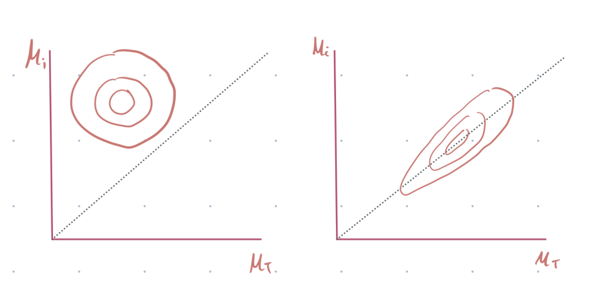
A centered parameterization implies that the subject-level parameters (\(i\)) are centered around the group-level parameter (\(T\)) as seen in equation 2. This makes sense, but it does not always work.
It will work well if their data is in abundance and they are highly heterogeneous. In this case, the group-level sigma will be large, and the posterior distribution space will be smooth. See fig 1, left below.
However, if the data are small, the group-level variance will be small, creating a situation where the subject-level parameters become very similar, and the posterior distribution space will be quite sharp. See figure 1, right below.
Why do we care about the posterior distribution geometry? HMC uses global step size independent of location in parameter space. Thus, a smooth geometry allows sampling accurately from the space, while a sharp geometry will probably lead to divergence or biased estimation of the group sigma.
A non-centered parameterization aims to resolve this issue by introducing an independent parameter Z (see equation 3 below) and using it to re-expresses the subject level parameters (without using (\(\mu_i\)). See equations 4&5.
- \[eq 3: Z_i \sim N(0,1)\]
- \[eq 4: \mu_i = \mu_T+Z_i *\sigma_T\]
- \[eq 5: x_i \sim N(\mu_T+Z_i *\sigma_T,\sigma_i)\]
This group of uncorrelated \(Z_i\) and \(\mu_T\) create a smooth space for the HMC sampler.
Check out this blog & this video for additional review on this topic.
Parameter transformations in stan
A common way to represent non-centered parameterization in Stan is via parameter transformation.
\(\mu_i\), as defined in equation 4, is a deterministic transformation of \(\mu_T\),\(Z_i\), and \(\sigma_T\), thus - it is not being sampled, but calculated.
Using a fast approximation of the unit normal cumulative distribution, we:
- Keeping all of the pre-transform parameters in approximately the same space (e.g., all sampled from a standard normal distribution) . This helps Stan with its gradient calculations – thereby speeding up the program.
- Bounding the pre-transform parameters into the range required by learning rates (or other parameters used), i.e. [0,1]. We can always scale a [0,1] bound parameter by multiplying/adding any value to it.
mu_i = Phi_approx(mu_T + sigma_T * Z_i);